Blob detection
CodeThe code is available here.
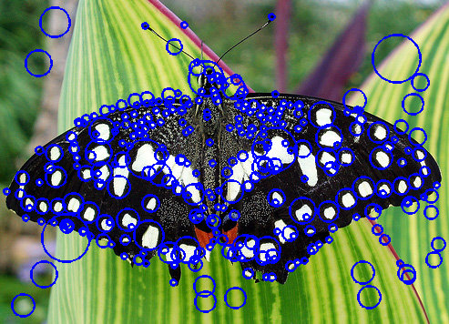
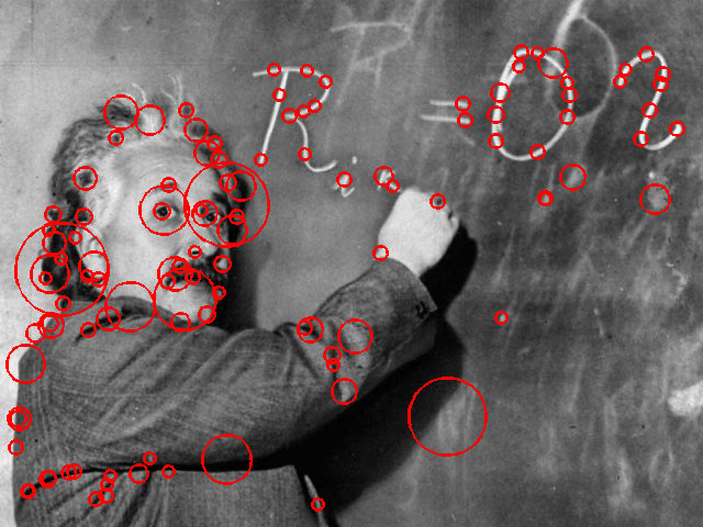
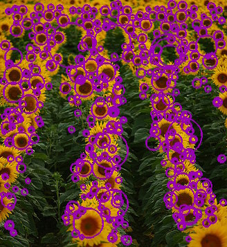
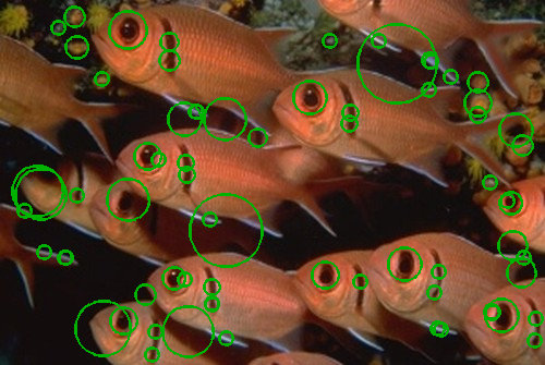
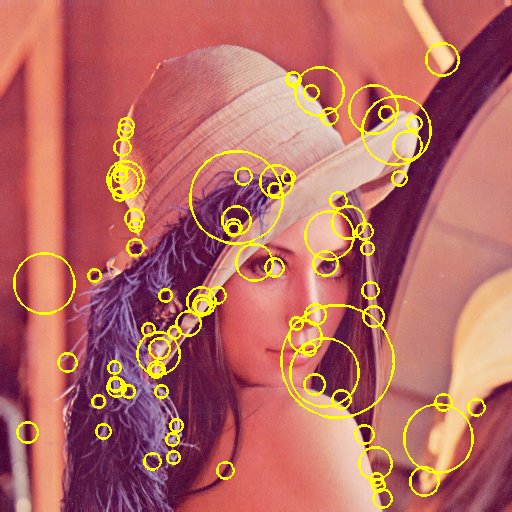
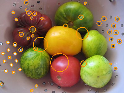
ImplementationThe blob detection works as described in class. A Laplacian of Gaussian filter is created. The image is then convolved with the filter while varying the relative size of the filter to the image size. This produces a 'stack' of several images convolved against Laplacians of increasing sizes. Each of the different filtered images has a different response for blobs of different sizes. All image scales are then filtered to suppress the nonmaximal responses. The gives a list of locations in each image where the response is a possible maximum. To test if the response is a real maximum, the location in the image is compared to the similar locations in the two scales immediately larger and immediately smaller. If the response is greater than both of those images, the blob must be about the size of the kernel that was used with the current image. If the response is not greater, perhaps the blob was scaled more to the size of the kernel in the larger or smaller image. Finally, after all images have been compared to their neighbors, the resulting maximum locations are marked as detected blobs.
Minor features
I have implemented an efficient blob detector that scales the image relative to the Laplacian kernel instead of creating a larger Laplacian for each image scale. As the relative size of the Laplacian to the image grows, the speed of the convolution increases, rather than decreasing.
The relative scale of the kernel to the image increases exponentially rather than linearly. This allows the smaller relative (where responses often change faster) to be sample more generously. As the kernel grows large compared to the image (say about >15%), the difference between responses in typical images does not change quickly. Therefore, it is better to sample the smaller relative sizes more often, as their values will change quickly.
When performing nonmaximum suppression between scaled images, the comparison window varies with the relative size of the Laplacian that was used to filter the image. Consider the case where the Laplacian was large compared to the image. Since the image was scaled to a small size and convolve, then resized, it is likely that the rescaled image was not scaled by a power of 2. Thus, the maximum locations between adjacent scale space images is likely to have shifted slightly. Since this shift is likely to increase as the relative size of the Laplacian increases, the comparison window grows to compensate.
Step size: As described above, I use an exponential step size. This is the result of my scale space containing many images that were very similar when the kernel is large relative to the image. Consider when relative size is linear from 1% to 30% in 30 steps. For an image of size 493x356, The first two scaled images go from 1800x1299 to 756x545- a very large change in numbers of pixels. The last step goes from 62x45 to 60x43- with the scale space results differing only slightly.
Maximum threshold: When performing nonmaximum suppression in each scale space slice, there is a threshold above which is a possible maximum and below is discarded. I chose to fix the threshold at 1000, as suggested in the harris code. I tried several other values, such as 10% of the max value in the slice and the mean of the values in the slice. A non-fixed threshold would result in low quality blobs around edges and such.
Max comparison window: I chose to have a varying comparison window for the 3d nonmaximum suppression. The reasons for this are explained above.
Scale range: Lastly, for each image, I decided on a minimum and maximum blob size to look for. This typically ranged from 1% or 3% to 30%. Searching for blobs smaller than 1% of the image size would result in long runtimes, as the image would be scaled very large to be relative to a kernel of reasonable resolution. The small results would often appear as noise without human recognizable blob sources. Values greater than 30% often resulted in detection of large shaded areas, if producing any results at all.
Mouse over the image to see the original image.
1.5% to 20%, in 20 steps
2% to 20%, in 20 steps
3% to 30%, in 30 steps
3% to 15%, in 20 steps
3% to 30%, in 20 steps
3% to 20%, in 20 steps
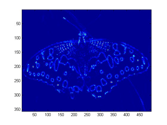
Also included is a sampling of the butterfly image as it was convolved with the Laplacian. These are the resulting scale space images.